Detecting Image Manipulation with a CNN

# Types of image alteration

In this project we distinguished between two kinds of changes:

1. Content tampering, such as replacing a face in Photoshop or changing text in a contract. Cropping, copying and removal account for many of these edits.
2. Image manipulation that can provide indirect evidence of tampering. Median filtering, Gaussian blur, added Gaussian noise and a second round of JPEG compression can all obscure traces of a content edit.

Ultimately we’d like to detect the first kind. That can require considerable expertise in forensics, photography and image analysis. Traditional methods might check noise consistency, geometry and lighting across each suspect region. Applying several checks to every region is time-consuming.

A machine-learning approach might segment the altered region directly, but training such a model isn’t straightforward. We could have generated as many examples as we liked by splicing images at random. But a model trained on crude composites might miss carefully retouched photos. Even a good score on equally crude test images would tell us little about that. Editing each photo by hand in Photoshop would take too long to produce enough training data.

That’s why our experiment focused on the second kind of alteration. We applied those operations to the original photos, labelled both the originals and the modified copies, trained a supervised convolutional network and measured its test accuracy after each epoch.

# Convolutional neural networks

# Why use a CNN?

Compared with a fully connected network. Here “DNN” refers to a deep network built from fully connected layers. A 1,000 × 1,000 RGB image already has three million input values. Connecting every value to every unit in the next layer quickly becomes expensive. The parameter count, resource use, risk of overfitting and possibility of getting stuck in a local optimum motivated our choice of a CNN.

A convolutional layer applies a small kernel to successive regions of the image to extract local features:

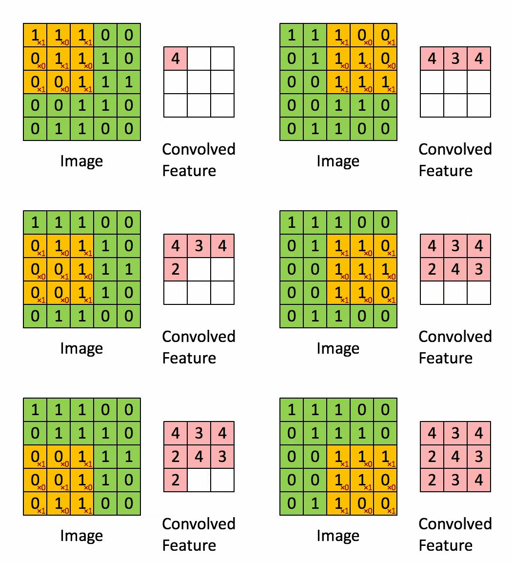
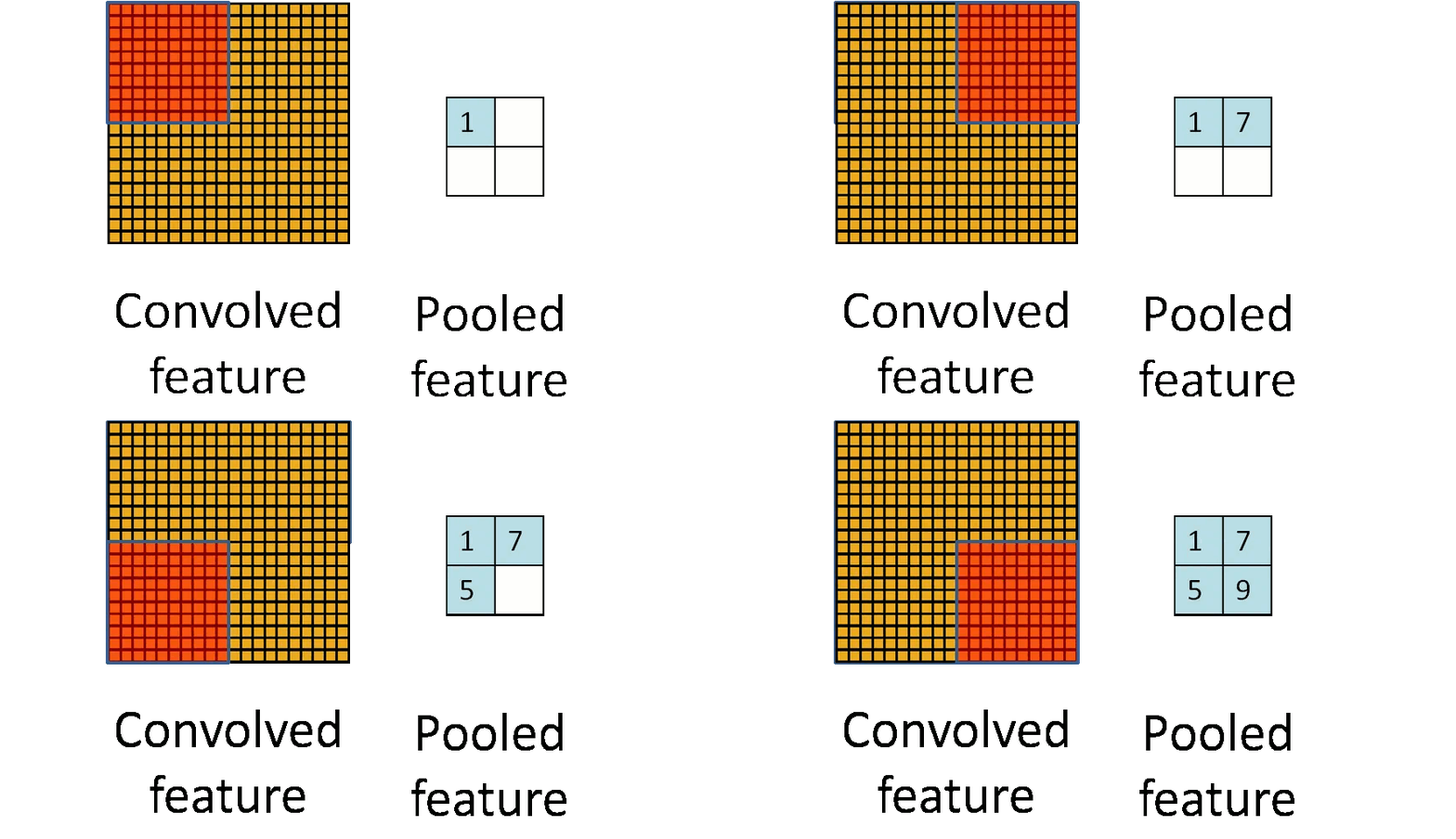
Even after convolution, the feature maps can be large. Pooling downsamples them. The example below uses a 10 × 10 sampling window on a 20 × 20 input to produce a 2 × 2 feature map:

Compared with hand-crafted forensic features. Traditional methods use image statistics and physical cues, particularly for copy-and-paste edits and splicing. The feature extractors we looked at involved a lot of hand-crafted calculations. We found their individual functions more complicated than the operations in our CNN. A CNN learns the features from examples, which was appealing when processing a large number of patches.

# Detecting the second kind of alteration

# Experimental data

We used 60 photos taken on phones: 40 for training and 20 for testing. We chose photos taken without beauty filters, because those filters are themselves a form of manipulation and could confound the labels. We deliberately included some blurry and tilted photos to cover more of the variation a model might encounter.

Using Python, OpenCV and NumPy, we produced five types of modified image: Gaussian blur, Gaussian noise, median blur, JPEG recompression, and changes in brightness or contrast. OpenCV’s GaussianBlur() and medianBlur() handled the two blurs; we wrote functions for the other operations. We included brightness and contrast because we suspected our network would struggle with them and wanted to test that prediction.

We kept both the originals and modified images, shuffled them together and kept each sample paired with its binary label. We extracted roughly 200,000 training patches and 100,000 test patches, each 28 × 28 pixels.

Our training setup:

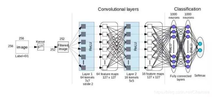
• Architecture: six convolutional layers in a simple VGG-style network, with pooling after each pair.
• Optimiser: Adam.
• Training: ten epochs.
• Learning rate: 1e-4 for the first five epochs and 1e-5 for the last five.
• Batch size: 50 samples.

# Results

For Gaussian blur, Gaussian noise, median blur and JPEG recompression, test accuracy settled above 90% after ten epochs. Gaussian noise reached 99%. Our guess was that its effect was particularly distinct from the original photos, making the pattern easier for the network to pick up across many examples.

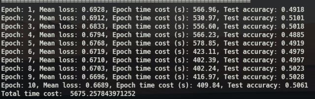
Brightness and contrast changes came in at around 50%. Our network couldn’t reliably distinguish these edits in this experiment. We suspect the features it learned from the modified patches remained too similar to those of the originals, but we didn’t verify that explanation.

Gaussian blur

Gaussian noise

Median blur

JPEG recompression

Brightness adjustment

Contrast adjustment