Applications: object detection and recognition, classification and retrieval, and super-resolution reconstruction.

Central question: how do we extract useful features?

---

# The architecture

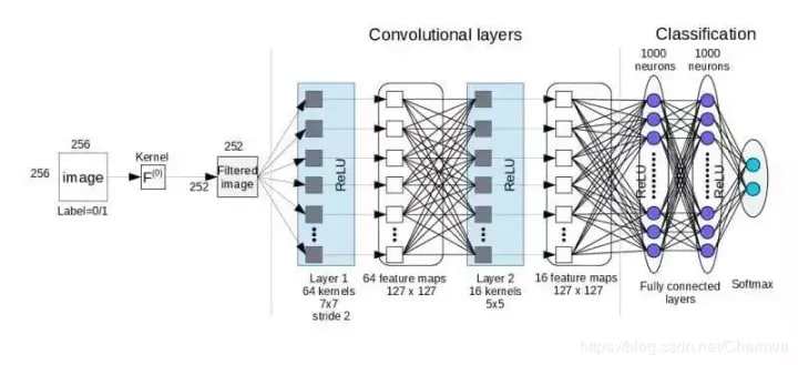
In the image classifier in these notes, the convolutional network accepts the image as a three-dimensional array of height, width and channels. The spatial structure is preserved at the input instead of immediately flattening the pixels.

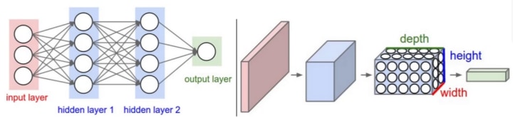
1. Input: the image array.
2. Convolution: extract local features.
3. Pooling: reduce the spatial size.
4. Fully connected layers: combine the features for prediction. Each output unit is connected to every unit in the preceding layer.

In the architecture shown, a ReLU activation follows each convolution. The convolution and pooling stages extract features; the classifier flattens the feature maps into a vector for the fully connected stage.

# Convolution

A filter combines local information across the input channels. If the input has $n$ channels, a conventional dense convolutional filter spans all $n$. Each filter produces one output feature map. With $m$ filters, the output has $m$ channels.

Four parameters are worth tracking:

1. Stride: how far the window moves at each step. A smaller stride samples positions more densely; 1 is common.
2. Kernel size: a smaller window examines a more local neighbourhood. A common choice is $3\times3$. A $1\times1$ kernel can mix channels at the same spatial location.
3. Padding: in a convolution without padding, central input values participate in more windows than edge values. Adding zeroes around the edges lets filters reach more boundary positions.
4. Number of filters: determines the number of output feature maps. Each filter learns its own weights.

When the stride divides the available distance exactly, the output dimensions are

• Height: $H_2=\frac{H_1-F_H+2P}{s}+1$.
• Width: $W_2=\frac{W_1-F_W+2P}{s}+1$.

Here $H_1,W_1$ are the input dimensions, $F_H,F_W$ the filter dimensions, $s$ the stride and $P$ the padding on each side. Convolution needn’t shrink the image: with suitable settings the output has the same height and width as the input.

# Pooling

Max pooling takes the largest value in each window. Average pooling takes its mean. Global average pooling averages the spatial positions in each channel. A pooling operation has no learned weight matrix, so it can be left out of a count of weight-bearing layers.

Downsampling loses some information. One common design choice is to increase the number of feature maps in the following convolution, for example by doubling it.

# Tracking feature map shapes

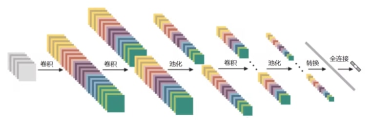
Convolution changes the features and can change the number of channels. Pooling reduces spatial dimensions. The final flattening step collects all the values from $n$ feature maps of width $w$ and height $h$ into a vector of length $w\times h\times n$.

# Residual networks

Does adding layers always improve a network? No. The middle layers extract features. Doing that fifty times needn’t give a better result than doing it twenty times. In the example below, the deeper network actually has higher training error.

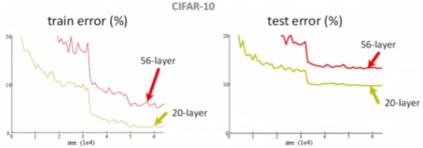
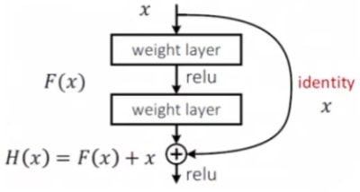
ResNet, proposed in 2015, addresses this with a residual connection. For matching input and output shapes, a residual block adds its input to the learned residual: $y=x+F(x)$. When $F(x)$ is close to zero, the block passes the input through nearly unchanged without having to learn the identity mapping from scratch.