# Decision trees

A decision tree classifies an observation through a sequence of tests. Training derives those decision rules from the examples.

Trees are fast to evaluate, and you can follow the tests to see which attributes mattered. Splitting on individual attributes can overlook relationships between them. An uneven class distribution can also affect performance.

# Building a tree

The central question is which attribute to test at each node.

Entropy measures uncertainty in the class distribution. In a dataset $D$ with $n_c$ classes, let $P(c_i)$ be the proportion in class $c_i$. Its entropy is

$Entropy(D)=-\sum_{i=1}^{n_c}P(c_i)\log_2P(c_i)$.

A pure node contains observations from a single class. One way to describe how close a node is to that state is the fraction covered by its majority class.

1. Choose a split. ID3 uses information gain, C4.5 uses gain ratio, and classification trees in CART use Gini impurity.
   • Information gain is the reduction in entropy after splitting on attribute $A$: $Gain(D,A)=Entropy(D)-\sum_{v=1}^V\frac{|D_v|}{|D|}Entropy(D_v)$. Here $V$ counts distinct values and $D_v$ is the subset with value $v$. The ratio $|D_v|/|D|$ weights each child by its size.
   • Information gain tends to favour attributes with many values, which can lead to overfitting. Gain ratio divides it by the entropy of the split: $Gain_{ratio}(D,A)=Gain(D,A)/H_A(D)$, where $H_A(D)=-\sum_{v=1}^V\frac{|D_v|}{|D|}\log_2\frac{|D_v|}{|D|}$.
   • Gini impurity is the probability that two independent draws from the class distribution differ. With class proportions $p_i$, $Gini(D)=1-\sum_{i=1}^k p_i^2$.
2. Partition the samples. The selected test assigns the observations to child nodes.
3. Repeat recursively. At each child choose a new split until a stopping condition applies, for example a pure node, no remaining attributes, or a maximum depth.
4. Assign leaves. Limits on leaf size, depth or purity can leave several classes in a leaf. Assign the most frequent class. In these notes, a tie is broken by choosing at random among the tied classes.
5. Prune. Removing overly complex branches can improve generalisation. Methods include reduced-error pruning (REP), pessimistic-error pruning (PEP), error-based pruning (EBP), cost-complexity pruning (CCP) and minimum-error pruning (MEP).
6. Predict. Follow the tests from the root to a leaf and return its class, or its numerical prediction for a regression tree.

# ID3

Compute the information gain for each candidate attribute and choose the largest. Create branches for its possible values. If no further split is possible, label the leaf with the most frequent class among its samples.

# C4.5

• Split selection. A low split entropy can inflate gain ratio. The selection heuristic first keeps attributes with above-average information gain and then chooses the highest gain ratio among them.
• Continuous attributes. ID3 handles discrete attributes. C4.5 can also split a continuous attribute by finding a threshold. Sort the distinct observed values. With $m$ values, there are $m-1$ midpoints between neighbours. Evaluate the information gain for each binary test (above the midpoint versus at or below it) and choose the best threshold.
• Missing values. Calculate gain among observations with known values and scale it by the proportion of observations with known values. If this attribute is used, distribute the weight of a sample with a missing value across children in proportion to the known samples in those branches.

# CART

CART builds binary trees for classification or regression. In the categorical classification example here, test whether attribute $A$ equals value $a$. The test divides $D$ into $D_1$ and $D_2$: samples with that value and all remaining samples. For each candidate split, weight each child’s Gini impurity by its share of the samples: $\frac{|D_1|}{|D|}Gini(D_1)+\frac{|D_2|}{|D|}Gini(D_2)$. Choose the split with the lowest weighted impurity. Every internal node has exactly two children.

# Anomaly detection

Anomaly detection looks for observations that don’t fit the expected pattern. One approach flags points with a low estimated probability density.

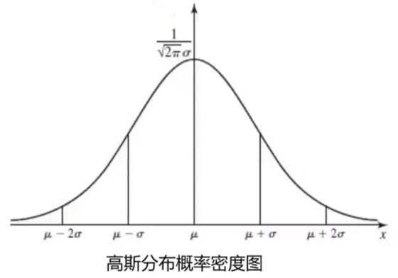
For a continuous variable, $p(x)$ describes density near $x$. The probability over an interval is $\int_{x_1}^{x_2}p(x)dx$, and the integral over the entire real line is 1.

Gaussian distribution

$$p(x)=\frac{1}{\sigma\sqrt{2\pi}}e^{-\frac{(x-\mu)^2}{2\sigma^2}}$$

The mean $\mu$ locates the centre. A larger standard deviation $\sigma$ spreads the distribution out. For $m$ observations the estimates used here are $\mu=\frac1m\sum_i x^{(i)}$ and $\sigma^2=\frac1m\sum_i(x^{(i)}-\mu)^2$.

Gaussian anomaly detection

For one-dimensional observations $x_1,\dots,x_m$, estimate the mean and standard deviation, calculate $p(x)$, and flag $x_i$ when $p(x_i)<\varepsilon$.

For $m$ samples with $n$ features, arrange the values by feature $j$ and observation $i$. Each row contains the $m$ observations for one feature:

$$\begin{bmatrix} x_1^{(1)} & \cdots & x_1^{(m)} \\ \vdots & & \vdots \\ x_n^{(1)} & \cdots & x_n^{(m)} \end{bmatrix}$$

Fit the Gaussian parameters separately for each feature:

$$\mu_j=\frac1m\sum_{i=1}^m x_j^{(i)},\qquad \sigma_j^2=\frac1m\sum_{i=1}^m(x_j^{(i)}-\mu_j)^2.$$

Under the independent-feature model, multiply the densities:

$$p(x)=\prod_{j=1}^n p(x_j)=\prod_{j=1}^n\frac{1}{\sigma_j\sqrt{2\pi}}e^{-\frac{(x_j-\mu_j)^2}{2\sigma_j^2}}.$$

Compare this joint density with the threshold $\varepsilon$.

# Principal component analysis

PCA projects high-dimensional data into fewer dimensions. The first principal direction captures the most variance. Each subsequent direction captures as much of the remaining variance as possible while staying orthogonal to the directions already chosen. PCA does not use class labels.

• Preprocess the features. For standardisation, centre them at zero and scale to unit standard deviation.
• Find the eigenvectors of the covariance matrix and the variance along each direction.
• Choose the target dimension $k$ based on the task or a desired fraction of explained variance.
• Project the observations onto the space spanned by the leading $k$ eigenvectors.

# Model optimisation checks

These notes consolidate an earlier post on model optimisation. They’re questions to investigate; the experiment determines which changes help.

# Data

Data quality limits what the model can achieve.

1. What does each feature mean? Removing irrelevant features can save computation and reduce overfitting.
2. Do the features have very different scales? Normalisation or standardisation can balance their influence and speed up convergence.
3. Are there outliers? Decide whether keeping or filtering them makes the model more robust.
4. Are there enough examples? Consider increasing the sample.
5. Does the collection method produce representative data?
6. Are labels assigned consistently under the same rules?

# Compare models

Try different models on comparable data and compare their performance to find one that better suits the task.

# Key parameters

Try every combination of the key parameter values under consideration and compare the model’s performance.