# Linear regression

# Logistic regression

Logistic regression is used for classification. There are two steps: choose the form of the decision boundary, then find the coefficients that minimise the loss.

The classification problem

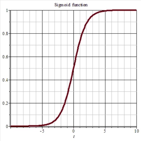
The sigmoid function $S(x)=\frac{1}{1+e^{-x}}$ maps a score to a value between zero and one. The curve is shown below. With a threshold of 0.5, values above the threshold are assigned class 1 and values below it class 0.

From a score to a probability

Write $P(x)=\frac{1}{1+e^{-g(x)}}$. The decision boundary is where $g(x)=0$. Taking $g(x)=x$ gives the sigmoid curve above; the same threshold rule applies.

A typical score has the form $g(x)=\theta_0+\theta_1x_1+\dots$. It can involve several variables and higher-order terms.

The loss function

The loss $J$ measures how well the prediction agrees with the label. It should be large for a confident wrong prediction and small for a confident correct one.

For a single observation, this gives

$\left.J_i=\left\{\begin{matrix}-\log\bigl(P(x_i)\bigr), &y_i=1\\-\log\bigl(1-P(x_i)\bigr), &y_i=0\end{matrix}\right.\right.$

Here $y_i$ is the true label and $P(x_i)$ is the predicted probability of class 1 for observation $x_i$.

For computation, the average loss over the dataset can be written as one expression:

$\begin{aligned}J&=\frac{1}{m}\sum_{i=1}^{m}J_{i}=-\frac{1}{m}\bigg[\sum_{i=1}^{m}\bigl(y_{i}\log\bigl(P(x_{i})\bigr)+(1-y_{i})\log\bigl(1-P(x_{i})\bigr)\bigr)\bigg]\end{aligned}$

Fitting the model

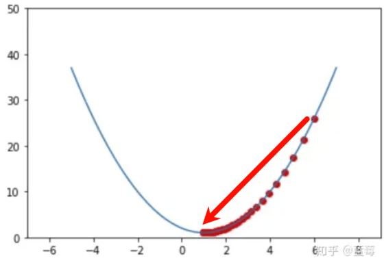
Use gradient descent to minimise the loss and find the coefficients $\theta_i$ of the decision boundary.

Here $j$ indexes the parameter and $t$ the iteration. The update for parameter $j$ is

$\theta_j^{(t+1)}=\theta_j^{(t)}-\alpha\left.\frac{\partial J}{\partial\theta_j}\right|_{\theta=\theta^{(t)}}$

Each update starts from the previous estimate and takes a step against the gradient. The step size is controlled by $\alpha$. With a suitable step size the estimates approach the minimum.